
When Detection is Perfect
When Every Target Within Some Distance is Detected
Imagine a line-transect study that collects counts of sighted targets and either total transect length or total number of observation points. Imagine further that target detectors (i.e., humans, cameras, etc.) detect every target out to a distance of w [m]. They do not miss any.
Note
For simplicity, this introduction focuses on line-transects. The same motivational themes apply to point counts along point-transects.
The data from such a study would fit in three columns, plus two cells, of a spreadsheet. The spreadsheet might like this,
| Transect | Length [m] | Number Seen |
|---|---|---|
| 1 | \(x_1\) | \(n_1\) |
| 2 | \(x_2\) | \(n_2\) |
| 3 | \(x_3\) | \(n_3\) |
The two additional cells are the width of the observed strip (w [m]) and study area size (A [m^2]).
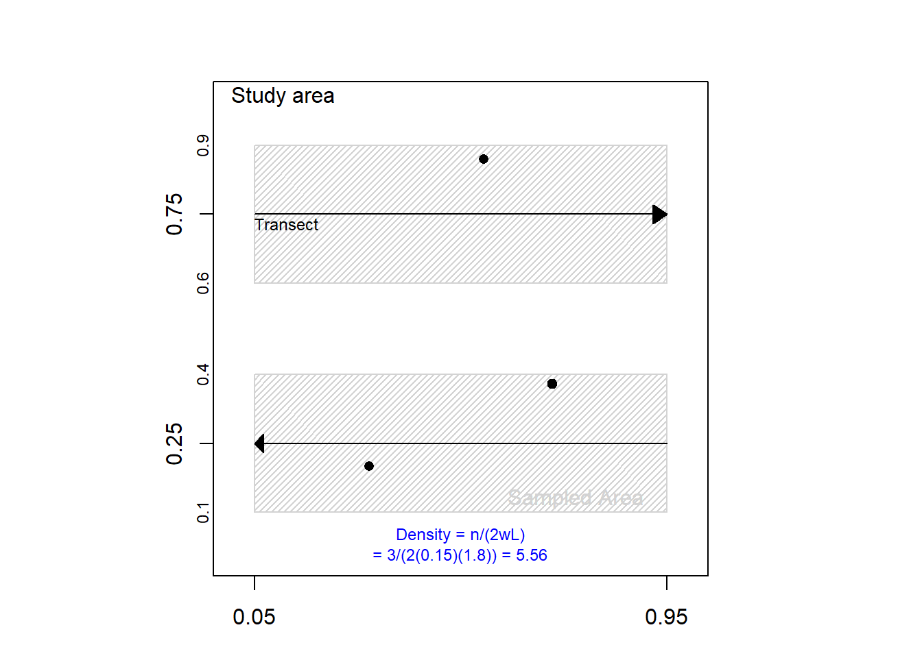
If detection of targets out to a distance of w is perfect, the counts, transect lengths, and w are sufficient to compute target density in the sampled area. In this case, density is simply the number of targets sighted divided by the sampled area, which under perfect detection is twice (assuming both sides of the transect are searched) the search width w times length of the transect (Figure 1).
TipSampled Area
Sampled area is the cumulative area (physical region) observed by target detectors during their transit of all transects.
When detection is perfect, density of targets on the sampled area is simply calculated as, \[ \hat{D} = \frac{n}{2wL} \tag{1}\] where \(n\) is total number of targets seen (sum of the third spreadsheet column), \(2w\) is width of the strip surveyed by the target detectors, and \(L\) is total length of transect traversed (sum of the second spreadsheet column).
NoteAside
The only random quantity in the equation for density is \(n\), the number of targets seen.
Once density is computed, abundance is, \[ N = A\hat{D} \tag{2}\] where \(A\) is total size of the region over which \(\hat{D}\) is thought to apply.
But, there is a problem.