Line Transects - No Covariates

Beginner

Author

Trent McDonald

Published

April 8, 2025

Modified

April 24, 2025

Abundance via line-transect distance-sampling when detection does not depend on covariates.

Construct the Rdistance data frame

library(Rdistance)

Loading required package: units

udunits database from C:/Users/trent/AppData/Local/R/win-library/4.4/units/share/udunits/udunits2.xml

Rdistance (v4.0.5)

# Example data (see ?sparrowDetectionData)
data("sparrowDetectionData")  # access example data
data("sparrowSiteData")
head(sparrowDetectionData)  # inspect data

  siteID groupsize sightdist sightangle     dist
1     A1         1        65         15 16.8 [m]
2     A1         1        70         10 12.2 [m]
3     A1         1        25         75 24.1 [m]
4     A1         1        40          5  3.5 [m]
5     A1         1        70         85 69.7 [m]
6     A1         1        10         90 10.0 [m]

head(sparrowSiteData)

  siteID  length observer bare herb shrub height shrubclass
1     A1 500 [m]     obs4 36.7 15.9  20.1   26.4       High
2     A2 500 [m]     obs4 38.7 16.1  19.3   25.0       High
3     A3 500 [m]     obs5 37.7 18.8  19.8   27.0       High
4     A4 500 [m]     obs5 37.7 17.9  19.9   27.1       High
5     B1 500 [m]     obs3 58.5 17.6   5.2   19.6        Low
6     B2 500 [m]     obs3 56.6 18.1   5.2   19.0        Low

# Make nested data frame required by Rdistance
sparrowDf <- RdistDf(sparrowSiteData
                     , sparrowDetectionData
                     , by = "siteID"
                     , pointSurvey = FALSE
                     , observer = "single"
                     , .detectionCol = "detections"
                     , .effortCol = "length")

Inspect the Rdistance data frame.

head(sparrowDf)

# A tibble: 6 × 9
# Rowwise:  siteID
  siteID         detections length observer  bare  herb shrub height shrubclass
  <fct>  <list<tibble[,4]>>    [m] <fct>    <dbl> <dbl> <dbl>  <dbl> <fct>     
1 A1               [15 × 4]    500 obs4      36.7  15.9  20.1   26.4 High      
2 A2               [13 × 4]    500 obs4      38.7  16.1  19.3   25   High      
3 A3               [10 × 4]    500 obs5      37.7  18.8  19.8   27   High      
4 A4               [14 × 4]    500 obs5      37.7  17.9  19.9   27.1 High      
5 B1                [1 × 4]    500 obs3      58.5  17.6   5.2   19.6 Low       
6 B3                [6 × 4]    500 obs1      56.8  18.4   7.5   19.7 Low

summary(sparrowDf, formula = dist ~ groupsize(groupsize))

Transect type: line
Effort:
       Transects: 72        
    Total length: 36000 [m] 
Distances:
   0 [m] to 207 [m]: 356
Sightings:
         Groups: 356 
    Individuals: 374

# see detections on transect A1
sparrowDf |> 
  dplyr::filter(siteID == "A1") |>
  dplyr::reframe(detections)

# A tibble: 15 × 5
   siteID groupsize sightdist sightangle dist
   <fct>      <int>     <int>      <int>  [m]
 1 A1             1        65         15 16.8
 2 A1             1        70         10 12.2
 3 A1             1        25         75 24.1
 4 A1             1        40          5  3.5
 5 A1             1        70         85 69.7
 6 A1             1        10         90 10  
 7 A1             1        15         85 14.9
 8 A1             1         5         20  1.7
 9 A1             1         4         90  4  
10 A1             1        10         85 10  
11 A1             1        10         80  9.8
12 A1             1        70         75 67.6
13 A1             1        75         80 73.9
14 A1             1        75         85 74.7
15 A1             1        30         45 21.2

# see detections on 5th transect
sparrowDf$detections[[5]]

# A tibble: 1 × 4
  groupsize sightdist sightangle dist
      <int>     <int>      <int>  [m]
1         1        13         25  5.5

Estimate hazard rate distance function

# First, set upper (right) truncation distance
whi <- set_units(200, "m")

# Fit hazard rate likelihood 
dfuncFit <- sparrowDf |>
  dfuncEstim(dist ~ groupsize(groupsize)
             , likelihood = "hazrate"
             , w.hi = whi)

# plot
plot(dfuncFit
   , nbins = 30
   , col = "dodgerblue"
   , border = NA)

Density and abundance: Point estimates

# First, set study area size or desired density base
oneHectare <- set_units(1, "ha")

# To save computation time, set `ci = NULL`
# to compute point estimates only, i.e., 
abunFit <- dfuncFit |>
  abundEstim(area = oneHectare
             , ci = NULL)

summary(abunFit)

Call: dfuncEstim(data = sparrowDf, dist ~ groupsize(groupsize),
   likelihood = "hazrate", w.hi = whi)
Coefficients:
             Estimate  SE         z          p(>|z|)     
(Intercept)  3.880324  0.1024185  37.886959  0.000000e+00
k            2.966557  0.3724577   7.964816  1.654703e-15

Convergence: Success
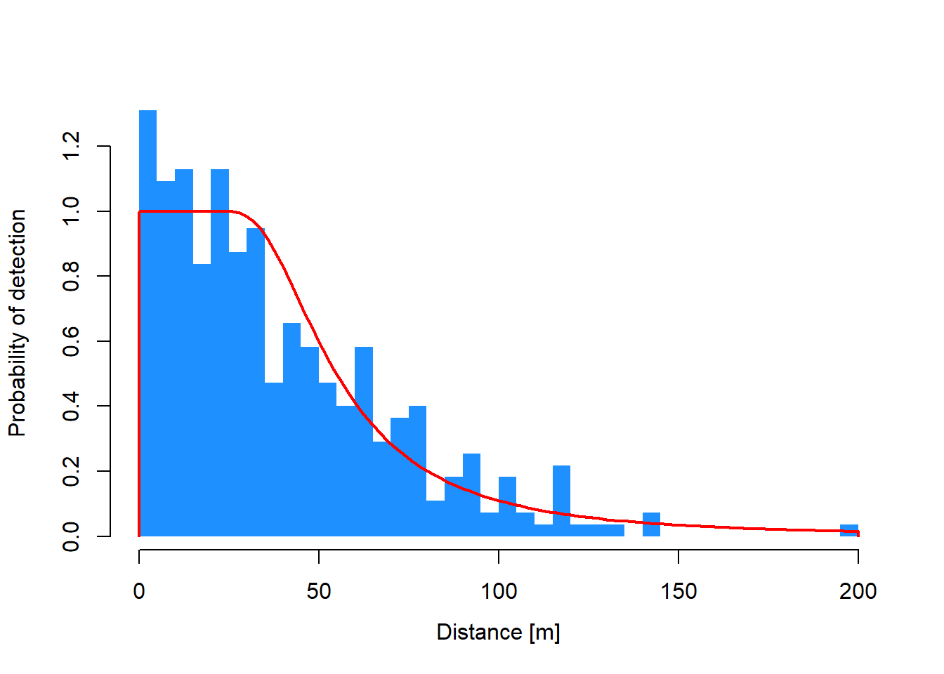
Function: HAZRATE  
Strip: 0 [m] to 200 [m] 
Effective strip width (ESW): 64.40993 [m] 
Probability of detection: 0.3220496
Scaling: g(0 [m]) = 1
Log likelihood: -1647.79 
AICc: 3299.614

     Surveyed Units: 36000 [m] 
   Individuals seen: 372 in 354 groups 
 Average group size: 1.050847 
   Group size range: 1 to 3 
Density in sampled area: 8.021538e-05 [1/m^2]
Abundance in 10000 [m^2] study area: 0.8021538

# Estimates are stored inside the output object
data.frame(abunFit$estimates)

        id X.Intercept.        k              density abundance nGroups nSeen
1 Original     3.880324 2.966557 8.021538e-05 [1/m^2] 0.8021538     354   372
         area surveyedUnits avgGroupSize avgEffDistance
1 10000 [m^2]     36000 [m]     1.050847   64.40993 [m]

Density and abundance: With confidence intervals

# Set `ci =` to desired confidence level
# Set `R =` to number of bootstrap iterations
abunFit <- dfuncFit |>
  abundEstim(area = oneHectare
             , ci = 0.95
             , R = 100)

summary(abunFit)

Call: dfuncEstim(data = sparrowDf, dist ~ groupsize(groupsize),
   likelihood = "hazrate", w.hi = whi)
Coefficients:
             Estimate  SE         z          p(>|z|)     
(Intercept)  3.880324  0.1024185  37.886959  0.000000e+00
k            2.966557  0.3724577   7.964816  1.654703e-15

Convergence: Success
Function: HAZRATE  
Strip: 0 [m] to 200 [m] 
Effective strip width (ESW): 64.40993 [m] 
Probability of detection: 0.3220496
Scaling: g(0 [m]) = 1
Log likelihood: -1647.79 
AICc: 3299.614

     Surveyed Units: 36000 [m] 
   Individuals seen: 372 in 354 groups 
 Average group size: 1.050847 
   Group size range: 1 to 3 

Density in sampled area: 8.021538e-05 [1/m^2]
                 95% CI: 6.156131e-05 [1/m^2] to 0.000119359 [1/m^2]

Abundance in 10000 [m^2] study area: 0.8021538
                             95% CI: 0.6156131 to 1.19359

Final density estimate (at the bottom of the output) is 0.8022 sparrows per hectare (95% CI: 0.6156 to 1.1936).

# Note: all bootstrap results are stored inside the output object
head(data.frame(abunFit$B))

             id X.Intercept.        k              density abundance nGroups
1 Bootstrap_001     4.015135 3.822332 8.869245e-05 [1/m^2] 0.8869245     415
2 Bootstrap_002     3.576244 2.429407 1.192291e-04 [1/m^2] 1.1922913     431
3 Bootstrap_003     4.016494 3.148473 6.210661e-05 [1/m^2] 0.6210661     308
4 Bootstrap_004     4.103457 3.907096 7.409921e-05 [1/m^2] 0.7409921     377
5 Bootstrap_005     3.855635 2.801255 8.402646e-05 [1/m^2] 0.8402646     368
6 Bootstrap_006     3.759147 2.500070 9.779088e-05 [1/m^2] 0.9779088     400
  nSeen        area surveyedUnits avgGroupSize avgEffDistance
1   436 10000 [m^2]     36000 [m]     1.050602   68.27588 [m]
2   447 10000 [m^2]     36000 [m]     1.037123   52.07061 [m]
3   322 10000 [m^2]     36000 [m]     1.045455   72.00880 [m]
4   395 10000 [m^2]     36000 [m]     1.047745   74.03738 [m]
5   388 10000 [m^2]     36000 [m]     1.054348   64.13324 [m]
6   430 10000 [m^2]     36000 [m]     1.075000   61.07136 [m]