The Two-Stage Approach: Modeling Abundance as a Function of Covariates

Author

Jason D. Carlisle and Trent L. McDonald

Published

April 26, 2025

Modified

April 26, 2025

Introduction

This tutorial builds on introductory material presented in the Beginner Line-transect Analysis tutorial. The beginner tutorial focused on generating an overall abundance estimate in a defined study area. The goal of many modern distance-sampling studies is to relate abundance to other variables. For example, the study may wish to describe habitat-associations of a species by relating local abundance to characteristics of the survey site (e.g., vegetation height), or to test for a difference in abundance among sites that received an experimental treatment (e.g., forest thinning vs control). At their core, these studies relate abundance to covariates, and distance-sampling really only serves as an initial step that accounts for imperfect detectability of the focal species.

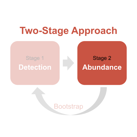
In the field of conventional distance-sampling (à la Buckland et al. 2001), the method that relates detectability-adjusted abundance to covariates has come to be known as the “two-stage” approach. The initial paper on this approach is Buckland et al. 2009, but Chapter 7 of Buckland et al. 2015 contains a nice comprehensive description.

Here, we illustrate the two-stage approach using the internal datasets sparrowSiteData and sparrowDetectionData that describe a line transect survey of Brewer’s Sparrow (Spizella breweri) in central Wyoming. The motivating research question was, “Are Brewer’s Sparrows more abundance in shrubbier habitats?” In short, we use Rdistance to produce site-level estimates of abundance corrected for imperfect and variable detection and model those estimates as a function of the amount of shrub cover associated with the transect using Poisson regression.

Note

This tutorial uses version 4.0.6 of Rdistance. Site-level abundance was difficult to estimate using previous versions.

Why the Two-Stage Approach?

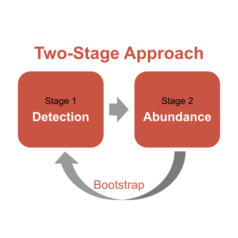
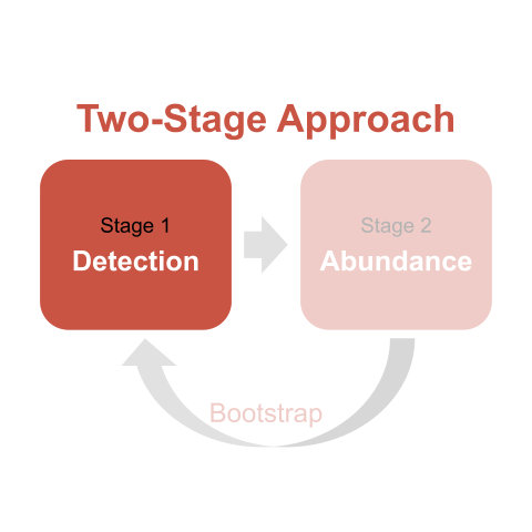
Carlisle and Chalfoun (2020) state that the number of sparrows counted at a site is the result of two processes: an ecological process affecting latent abundance (latent because it is incompletely observed due to detection error; Kéry and Schaub 2012) and an observation process that produces counts of latent abundance when probability of detection < 1 (Kéry and Schaub 2012). The two-stage approach provides the flexibility to model each process independently and (when done correctly with a bootstrap – more on that later) incorporates the uncertainty in estimating both processes into the final results (Buckland et al. 2009, 2015). The first stage estimates detection probability (often, but not necessarily always) in relation to covariates and generates site-specific estimates of sparrow density. This stage adjusts counts for imperfect and variable detection arising at different sites. The second stage models those estimated sparrow densities in relation to other variable(s) of interest (often, but not necessarily always) using some form of a regression model. As illustrated in the diagram above, what happens in the 2nd stage depends on what happened in the 1st stage. Or, a statistician might say that abundance estimates are conditional on detectability estimates.

Although outside the scope of this tutorial, users should be aware that hierarchical distance-sampling models (made popular by R package unmarked, Fiske and Chandler 2011, Kellner et al. 2023) make use of an integrated or unconditional likelihood, meaning the detection and abundance processes are estimated in one model that accounts for uncertainty at both stages without requiring the bootstrap method we apply in this tutorial. See Kéry and Schaub 2012 and Kéry and Royle 2016 for more details.

Analyses that require the two-stage distance analysis approach.
Covariates in Detection Model	Covariates in Abundance Model	Approach
No	No	Basic
Yes	No	Basic
No	Yes	Two-Stage
Yes	Yes	Two-Stage

The Rdistance workflow of the two-stage approach proceeds as follows:

Model detection (abbreviated $p$ ) as function of the observer conducting the survey (to control for observer-level differences in sparrow detectability).
Model abundance (abbreviated $N$ ) as a function of shrub cover at the site (to answer the research question stated earlier).

In equation form, we model

$p \sim o b s e r v e r$

$N \sim s h r u b$

1 Preliminaries

1.1 Install and load Rdistance

If not already, the latest version of Rdistance needs to be installed. In the R console, issue install.packages("Rdistance"). After installation, Rdistance will be loaded and ready to run in the current session after issuing the following:

require(Rdistance)

Loading required package: Rdistance

Loading required package: units

udunits database from C:/Users/trent/AppData/Local/R/win-library/4.4/units/share/udunits/udunits2.xml

Rdistance (v4.0.6)

We also load an additional package to aid this tutorial:

require(dplyr, warn.conflicts = FALSE)

Loading required package: dplyr

1.2 Read the input data

For this tutorial, we use example data included with Rdistance from a survey of Brewer’s Sparrow abundance in relation to site-specific habitat conditions in central Wyoming (Carlisle and Chalfoun 2020, see help("sparrowSiteData") for additional details).

The first dataset, sparrowSiteData, is a data.frame with one row for each of 72 transects surveyed, and the following important columns (in addition to others not used in this tutorial):

siteID = Factor (72 levels), the site or transect surveyed.
length = Numeric, the length (m) of each transect.
observer = Factor (5 levels), identity of the observer who surveyed the transect.
shrub = Numeric, the mean shrub cover (%) within 100 m of the transect.

Load and view the first 6 lines of the sparrow transects dataframe (sparrowSiteData) using the following commands:

data("sparrowSiteData")
head(sparrowSiteData)

  siteID  length observer bare herb shrub height shrubclass
1     A1 500 [m]     obs4 36.7 15.9  20.1   26.4       High
2     A2 500 [m]     obs4 38.7 16.1  19.3   25.0       High
3     A3 500 [m]     obs5 37.7 18.8  19.8   27.0       High
4     A4 500 [m]     obs5 37.7 17.9  19.9   27.1       High
5     B1 500 [m]     obs3 58.5 17.6   5.2   19.6        Low
6     B2 500 [m]     obs3 56.6 18.1   5.2   19.0        Low

The second dataset, sparrowDetectionData, is a data.frame containing one row for each of the 356 groups of sparrows detected while surveying the transects described in sparrowSiteData. Important columns in this data frame are:

siteID = Factor (72 levels), the site or transect where the detection was made.
groupsize = Numeric, the number of individuals within the detected group.
dist = Numeric, the perpendicular, off-transect distance (m) from the transect to the detected group.

Load the example dataset of sparrow detections (sparrowDetectionData) using the following commands:

data("sparrowDetectionData")
head(sparrowDetectionData)

  siteID groupsize sightdist sightangle     dist
1     A1         1        65         15 16.8 [m]
2     A1         1        70         10 12.2 [m]
3     A1         1        25         75 24.1 [m]
4     A1         1        40          5  3.5 [m]
5     A1         1        70         85 69.7 [m]
6     A1         1        10         90 10.0 [m]

Zero transects

While siteID in sparrowDetectionData has 72 levels, one for each transect, sparrows were only sited on 61 transects. Eleven transects were so-called “zero” transects and their siteID do not appear in sparrowDetectionData.

The final step in data preparation is to make an ‘Rdistance data frame’ or RdistDf. ‘Rdistance data frames’ are nested data frames that contain site and detection information in one object. To do this, execute the ‘Rdistance data frame’ constructor function RdistDf, making sure to specify the primary key linking the two data frames (siteID) set pointSurvey to FALSE (since this was a line transect survey), and specify which column in sparrowSiteData contains the length of each transect (which indicates the survey effort, which in turn specifies the covered area).

sparrowData <- RdistDf(transectDf = sparrowSiteData,
                       detectionDf = sparrowDetectionData,
                       by = "siteID",
                       pointSurvey = FALSE,
                       .effortCol = "length")

The summary method provides a final check of the data.

summary(sparrowData,
        formula = dist ~ groupsize(groupsize))

Transect type: line
Effort:
       Transects: 72        
    Total length: 36000 [m] 
Distances:
   0 [m] to 207 [m]: 356
Sightings:
         Groups: 356 
    Individuals: 374

2 The Wrong Way

Analysts may be tempted to simply regress the number of observed sparrows onto covariates without adjusting for detectability. We run this ‘wrong’ analysis so that we can compare it to the ‘correct’ analysis later.

First, the ‘wrong’ analysis tallies the number of sparrows observed on each transect and plots them against sagebrush cover associated with each transect.

observedData <- sparrowData |>
  unnest() |>
  group_by(siteID) |>
  summarize(shrub = unique(shrub),
            individualsSeen = sum(groupsize)) |>
  mutate(individualsSeen = if_else(is.na(individualsSeen), 0, individualsSeen))

head(observedData)

# A tibble: 6 × 3
  siteID shrub individualsSeen
  <fct>  <dbl>           <dbl>
1 A1      20.1              15
2 A2      19.3              14
3 A3      19.8              10
4 A4      19.9              15
5 B1       5.2               1
6 B2       5.2               0

plot(individualsSeen ~ shrub,
     data = observedData,
     xlab = "Sagebrush Cover (%)",
     ylab = "Sparrow Count")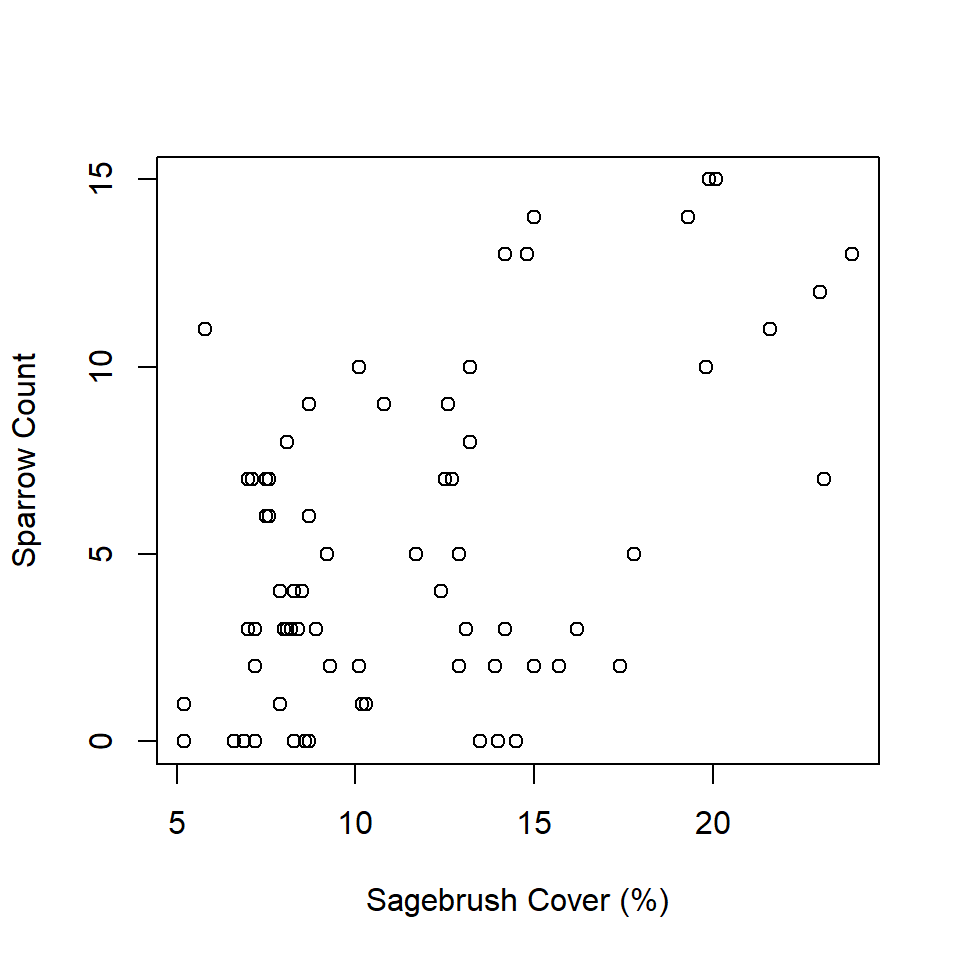

Second, the ‘wrong’ approach estimates a simple linear regression model to describe the relationship between sagebrush cover and number of sparrows.

mod <- lm(individualsSeen ~ shrub,
          data = observedData)

summary(mod)


Call:
lm(formula = individualsSeen ~ shrub, data = observedData)

Residuals:
    Min      1Q  Median      3Q     Max 
-6.5912 -3.1545 -0.2848  2.7734  8.3821 

Coefficients:
            Estimate Std. Error t value Pr(>|t|)    
(Intercept) -0.03103    1.17132  -0.026    0.979    
shrub        0.45671    0.09484   4.816  8.2e-06 ***
---
Signif. codes:  0 '***' 0.001 '**' 0.01 '*' 0.05 '.' 0.1 ' ' 1

Residual standard error: 3.743 on 70 degrees of freedom
Multiple R-squared:  0.2488,    Adjusted R-squared:  0.2381 
F-statistic: 23.19 on 1 and 70 DF,  p-value: 8.198e-06

plot(individualsSeen ~ shrub,
     data = observedData,
     xlab = "Sagebrush Cover (%)",
     ylab = "Sparrow Count (+/- 95% CI)")

predData <- data.frame(shrub = seq(min(observedData$shrub),
                                   max(observedData$shrub),
                                   length.out = 25))

predData <- cbind(predData,
                  predict(mod,
                          predData,
                          interval = "confidence",
                          level = 0.95))

lines(predData$shrub, predData$fit, col = "red", lwd = 3)
lines(predData$shrub, predData$lwr, col = "red", lwd = 2, lty = "dashed")
lines(predData$shrub, predData$upr, col = "red", lwd = 2, lty = "dashed")

But what’s wrong with that approach?

First and foremost, observers do not detect all sparrows during surveys, so the observed count of sparrows is lower than the true number of sparrows. It may be tempting to just treat the observed count as a meaningful index of abundance and stick with this approach, but that is problematic for reasons described by Marques et al. (2017) and Gu and Swihart (2004), namely bias in the density and the regression coefficient estimates. Second and less germane to this tutorial, a simple linear regression isn’t likely the most-appropriate form of regression model when responses are count data.

In the next section, we move on and extend this ‘wrong’ analysis using Rdistance to adjust for detection probability, then use detectability-adjusted sparrow density as the response variable (accomplished via a regression offset term - more on that later) in a Poisson generalized linear model (GLM).

3 The Right Way

3.1 Stage 1 - Estimate detection and site-level abundance

During stage one, we fit a distance function using Rdistance that will estimate detectability as a function of the observer who surveyed the transect. Observers are often a key source of detection heterogeneity in wildlife surveys (Schmidt et al. 2023).

dfunc <- dfuncEstim(formula = dist ~ observer + groupsize(groupsize),
                    data = sparrowData,
                    likelihood = "halfnorm",
                    w.hi = set_units(100, "m"),
                    outputUnits = "m")

newdata <- data.frame(observer = unique(sparrowData$observer))
plot(dfunc,
     newdata = newdata)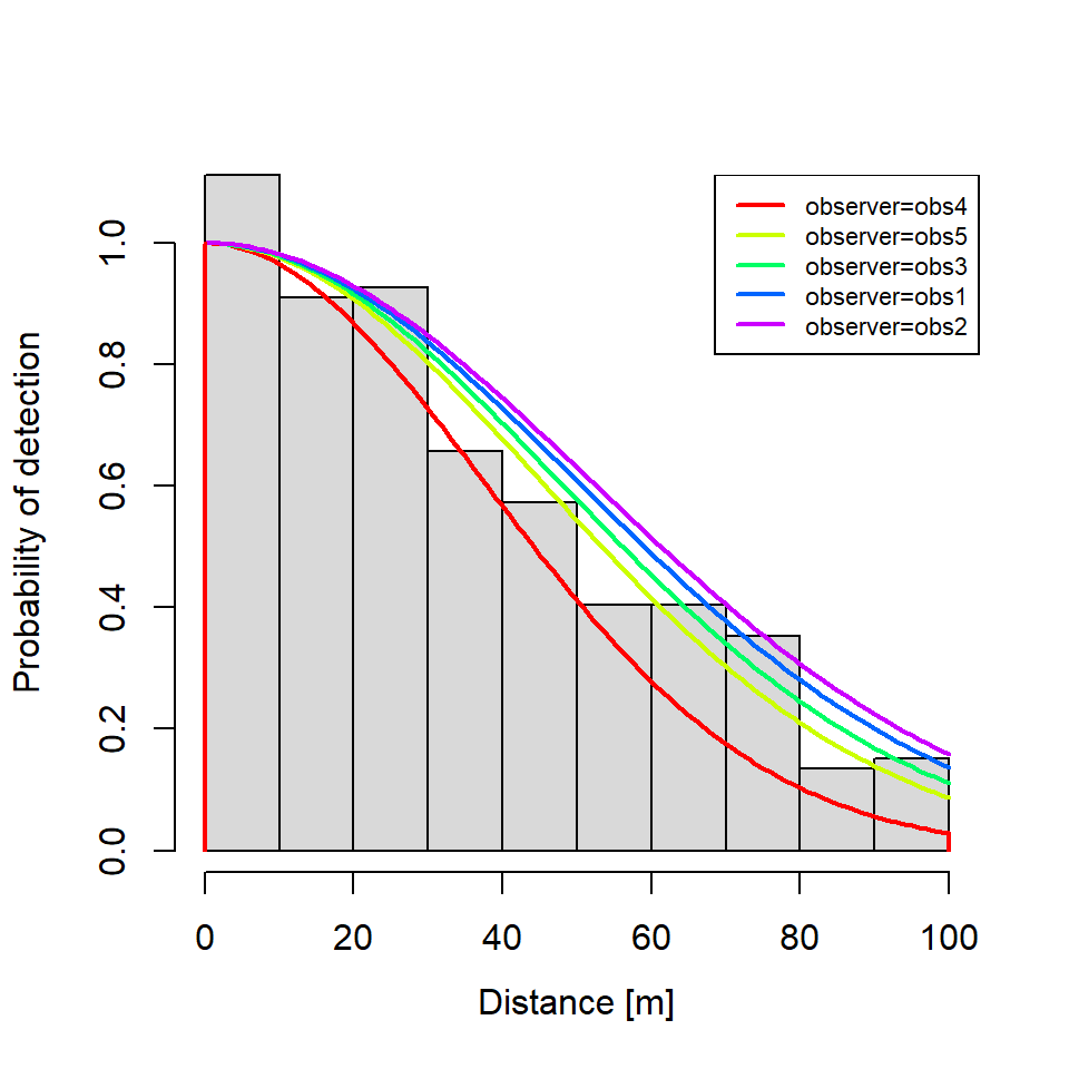

Figure 1: Off-transect observation distances of sparrows as a function of observer.

Next, we produce estimates of abundance on each transect. This step is a departure from the beginner tutorial, and is necessary because detectability varies among trancects and these transect-level abundance estimates become the response variable in a regression model during stage 2 of the two-stage approach.

abundBySite <- predict(dfunc,
                       type = "abundance")

# Explore output
head(abundBySite)

# A tibble: 6 × 6
  siteID individualsSeen avgPdetect abundance   density effort
  <fct>            <dbl>      <dbl>     <dbl>   [1/m^2]  [m^2]
1 A1                  15      0.467     32.1  0.000321  100000
2 A2                  14      0.467     30.0  0.000300  100000
3 A3                  10      0.552     18.1  0.000181  100000
4 A4                  14      0.552     25.3  0.000253  100000
5 B1                   1      0.576      1.74 0.0000174 100000
6 B2                   0      0.576      0    0         100000

These are the columns in this new abundBySite data frame:

siteID = the site or transect surveyed.
individualsSeen = total sparrows observed at this site (on this transect) within the truncation distance we specified when calling dfuncEstim. In this case, the sum of group sizes for groups detected within 100 m of the transect.
avgPdetect = average probability of detection for all groups detected at this site. In this case, probability of detection depends only on the observer who surveyed the site.
abundance = number of sparrows at each site (see effort for how the size of each site is defined), after adjusting for detection probability. In this case, abundance = individualsSeen / avgPdetect because one observer surveyed each site and detection probability is constant across detections of a single site. If detection depends on detection-level covariates (such as sex, color, or size), abundance will be the sum of adjusted counts across detections at a single site (i.e., sum(groupsize/pDetect) over groupsizes detected on the transect).
density = density of sparrows at each site (see effort for the size of each site), after adjusting for detection probability; abundance / effort.
effort = size of the area surveyed at each site. In this case, each site was 500 m long, with a truncation distance of 100 m, and both sides of the transect were surveyed; i.e., 500 m * 100 m * 2 = 100,000 m^2 or 10 ha.

Note that the density and effort columns have defined units. Here, these are based on meters (m), because we specified outputUnits = "m" when we fit the detection model using dfuncEstim. Density of sparrows per square meter is really small and hard to interpret. Instead, let’s use the units package to convert density and effort into something more digestible. Square kilometers is a decent option, but songbird biologists are a strange lot and often think in hectares (ha). For the unitiated, 1 ha = 100 m * 100 m).

abundBySite <- abundBySite |>
  mutate(density = set_units(density, "1/ha"),
         effort = set_units(effort, "ha"))

head(abundBySite)

# A tibble: 6 × 6
  siteID individualsSeen avgPdetect abundance density effort
  <fct>            <dbl>      <dbl>     <dbl>  [1/ha]   [ha]
1 A1                  15      0.467     32.1    3.21      10
2 A2                  14      0.467     30.0    3.00      10
3 A3                  10      0.552     18.1    1.81      10
4 A4                  14      0.552     25.3    2.53      10
5 B1                   1      0.576      1.74   0.174     10
6 B2                   0      0.576      0      0         10

Lastly, we append the site-level covariates to abundBySite in preparation for stage 2.

abundBySite <- abundBySite |>
  left_join(sparrowSiteData,
            join_by(siteID))

head(abundBySite)

# A tibble: 6 × 13
  siteID individualsSeen avgPdetect abundance density effort length observer
  <fct>            <dbl>      <dbl>     <dbl>  [1/ha]   [ha]    [m] <fct>   
1 A1                  15      0.467     32.1    3.21      10    500 obs4    
2 A2                  14      0.467     30.0    3.00      10    500 obs4    
3 A3                  10      0.552     18.1    1.81      10    500 obs5    
4 A4                  14      0.552     25.3    2.53      10    500 obs5    
5 B1                   1      0.576      1.74   0.174     10    500 obs3    
6 B2                   0      0.576      0      0         10    500 obs3    
# ℹ 5 more variables: bare <dbl>, herb <dbl>, shrub <dbl>, height <dbl>,
#   shrubclass <fct>

We now have a site-level data frame with detection-stage modeling results on the same row as our site-level covariates, and we are ready to proceed to stage 2 of the two-stage approach.

3.2 Stage 2 - Relate abundance to covariates using a GLM

The first step in understanding stage 2 of the two-stage approach is to understand regression model offset terms. Here’s a brief crash-course, but see Section 9.11.1 of Zuur et al. 2009 for a more-detailed explanation.

Offset terms are the denominators for response variables. For example, if 5 sparrows were counted on a 10 ha site, we could model sparrow density (0.5 birds / ha) by treating the count (5) as the response variable and surveyed area (10 ha) as the offset term. This separation of the count and area surveyed is preferable to simply treating density itself as the response variable and forgoing the offset term because regression models that are well-suited for modeling abundance processes (i.e., so-called count regression models like Poisson or Negative Binomial GLMs and their extensions) cannot accommodate non-integer values in the response variable. So although a Poisson GLM cannot accept 0.5 birds / ha directly as a response variable value, it is more than happy to accept 5 birds counted (response variable) per 10 ha surveyed (offset term), which is equivalent.

So, here we add an offsetTerm column that holds the appropriate value that will produce detection-adjusted density when the number of individuals detected (individualsSeen column) is the numerator. We’ve already established that the effort column needs to figure into the offset term to represent the area surveyed; but don’t forget that the number of individuals detected needs to be inflated according to the detection probability too. We can accomplish both by using the product of avgPdetect and effort as the offset term. Note that the glm package needs the units to be stripped away from the offset term, hence the need for as.numeric.

abundBySite <- abundBySite |>
  mutate(offsetTerm = as.numeric(avgPdetect * effort))

head(abundBySite)

# A tibble: 6 × 14
  siteID individualsSeen avgPdetect abundance density effort length observer
  <fct>            <dbl>      <dbl>     <dbl>  [1/ha]   [ha]    [m] <fct>   
1 A1                  15      0.467     32.1    3.21      10    500 obs4    
2 A2                  14      0.467     30.0    3.00      10    500 obs4    
3 A3                  10      0.552     18.1    1.81      10    500 obs5    
4 A4                  14      0.552     25.3    2.53      10    500 obs5    
5 B1                   1      0.576      1.74   0.174     10    500 obs3    
6 B2                   0      0.576      0      0         10    500 obs3    
# ℹ 6 more variables: bare <dbl>, herb <dbl>, shrub <dbl>, height <dbl>,
#   shrubclass <fct>, offsetTerm <dbl>

Next, we estimate a Poisson GLM to model the relationship between shrub cover and detectability-adjusted sparrow density. As one further complication, because Poisson GLMs use a log link function by default, it is imperative to apply log to your offset term either when you create it (which we did not do above), or when you specify the regression formula in your call to glm (which we do below).

pmod <- glm(individualsSeen ~ shrub + offset(log(offsetTerm)),
            data = abundBySite,
            family = "poisson")

summary(pmod)


Call:
glm(formula = individualsSeen ~ shrub + offset(log(offsetTerm)), 
    family = "poisson", data = abundBySite)

Coefficients:
             Estimate Std. Error z value Pr(>|z|)    
(Intercept) -1.189401   0.143634  -8.281   <2e-16 ***
shrub        0.082838   0.009892   8.375   <2e-16 ***
---
Signif. codes:  0 '***' 0.001 '**' 0.01 '*' 0.05 '.' 0.1 ' ' 1

(Dispersion parameter for poisson family taken to be 1)

    Null deviance: 291.90  on 71  degrees of freedom
Residual deviance: 227.51  on 70  degrees of freedom
AIC: 435.48

Number of Fisher Scoring iterations: 5

After backtransforming using the inverse of th log link, we see that the estimated density of Brewer’s Sparrows increases by a multiplicative 1.09 for every incremental 1% increase in shrub cover at a site.

exp(coef(pmod))

(Intercept)       shrub 
  0.3044034   1.0863656

We visualize the relationship and accompanying 95% CIs as follows. Note the requirement to provide a value for the offset term in the call to predict. By specifying offsetTerm = 1, we’re predicting the density of sparrows per 1 ha, which matches the scale at which we calculated density in abundBySite, allowing us to plot the scatterplot of points behind the estimated regression line.

predData <- data.frame(shrub = seq(min(abundBySite$shrub),
                                   max(abundBySite$shrub),
                                   length.out = 25),
                       offsetTerm = 1)

predData <- cbind(predData,
                  predict(pmod,
                          predData,
                          type = "link",
                          se.fit = TRUE))

predData <- predData |>
  mutate(densityEst = exp(fit),
         lwr = exp(fit - 1.96 * se.fit),
         upr = exp(fit + 1.96 * se.fit))

plot(abundBySite$density ~ abundBySite$shrub,
     xlab = "Shrub Cover (%)",
     ylab = "Sparrow Density (birds/ha)")
lines(predData$shrub, predData$densityEst, col = "red", lwd = 3)
lines(predData$shrub, predData$lwr, col = "red", lwd = 2, lty = "dashed")
lines(predData$shrub, predData$upr, col = "red", lwd = 2, lty = "dashed")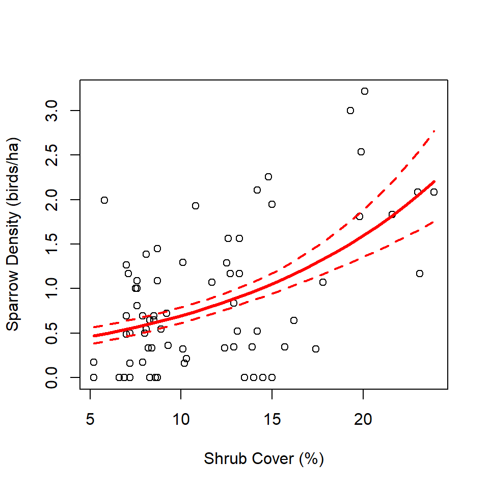

Figure 2: Detection-adjusted sparrow density as a function of scrub percentage on the transect, with (incorrectly small) 95% confidence intervals.

Great! That answers our research question, right? Sparrows are more abundant in shrubbier sites, and we accounted for variable detection probabilities among observers. But, are the confidence intervals accurate? Did we account for all sources of variation?

We didn’t. The last issue in our analysis is that the offset term is a quantity derived from the detection model and hence is random variable with uncertainty (think confidence intervals [CIs]). We estimated the offset term. We do not know its true value. This is a problem because regression models treat the offset term as a constant, which means that this Poisson regression model swept some uncertainty under the rug and our results were artificially precise (Buckland et al. 2009). In other words, the CIs on the regression plot are artificially too tight. The solution to this last issue is to re-do the analysis in a way that gives an honest accounting of the uncertainty inherent in both the detection and abundance stages of the analysis. The answer here is the bootstrap.

3.3 Bootstrap both stages to propagate uncertainty

Bootstrapping is a general approach to generate confidence intervals without relying on parametric assumptions, and it works by re-sampling the input data with replacement, then re-running the analysis.

The story goes that Efron (1979) named the method “bootstrapping” to invoke the imagery of a person pulling themselves out of mud by their bootstraps (Manly and Navarro Alberto 2020). In that same vein, a sample of data can make inference to the population from whence it came, simply based on its own merits and absent any other information.

Here, we use a for loop to re-sample our data and re-run our analysis a bunch of times. The primary step is to re-sample the sites (transects) with replacement to form a ‘bootstrap sample’, then repeat stages 1 and 2 of the analysis on that bootstrap sample of sites (and accompanying detections). Within each iteration of the bootstrap routine, a different collection of sites is selected, meaning a different set of detections is analyzed. Because the sampling is done with replacement, any given site (and its accompanying detections) may appear in a bootstrap sample once, multiple times, or not at all. Because of this resampling, the estimate of detection probability for a given site will vary from iteration to iteration, meaning the value of the offset term will also vary from iteration to iteration, thus propagating uncertainty from the stage 1 detection model to the stage 2 abundance model.

dplyr

The following code block makes heavy use of dplyr and its syntax. In particular, it uses left_join to expand a transect’s detections multiple times if the transect is re-sampled multiple times. The expansion is accomplished by calling left_join with the nested (detection) data frame to avoid a many-to-many join. Readers unfamiliar with dplyr and joins may have difficulty interpreting the code.

# Number of bootstrap iterations
# Consider a few hundred or few thousand for production-level analyses
R <- 100  

# Empty vectors to store the coefficient estimates from the GLM
b0 <- rep(NA, R)
b1 <- rep(NA, R)

# Condensed (nested) version of detection data, 1 row per transect
# (for merging with sites)
nestedDetectionData <- sparrowDetectionData |> 
  nest_by(siteID)

# Bootstrap loop
for (i in 1:R) {
  
  # Sample rows, with replacement, from site data
  new.sparrowSiteData <- sparrowSiteData |>
    slice_sample(prop = 1,
                 replace = TRUE)
  
  # Once during the tutorial, examine which sites made 
  # it into the bootstrap sample. Note: some of these are 
  # so-called "zero" transects, which is what we want.
  if( i <= 1) {
    cat(paste0("---- Sites in Bootstrap ", i, "\n"))
    print(table(new.sparrowSiteData$siteID))
  }
  
  # Some site appear multiple times, so assign a new, unique siteID
  # b/c Rdistance requires unique site names. Site A1 is named A1.1
  # the first time it is selected, A1.2 the second, etc. Preserve
  # original siteID for merging later.
  new.sparrowSiteData <- new.sparrowSiteData |> 
    group_by(siteID) |> 
    mutate(siteIDBoot = paste(siteID, row_number(), sep = ".")) |> 
    ungroup() |> 
    arrange(siteIDBoot) |> 
    dplyr::select(siteIDBoot, everything())
  
  if( i <= 1){
    cat(paste0("---- New Site Data (iteration ", i, ")\n"))
    print(head(new.sparrowSiteData))
  }
  
  # Compile the detection data from the bootstrap sample
  # If site A1 is represented once in the bootstrap sample, 
  # all detections at A1 should be included once
  # If twice, all detections included twice, etc.
  
  new.sparrowDetectionData <- nestedDetectionData |>
    left_join(new.sparrowSiteData, by = "siteID") |>
    filter(!is.na(siteIDBoot)) |> # drop un-bootstrap sampled transects
    dplyr::ungroup() |> 
    select(siteIDBoot, data) |> 
    tidyr::unnest(cols = "data") # 'tidyr::' b/c don't want Rdistance::unnest

  if( i <= 1){
    cat(paste0("---- New Detection Data (iteration ", i, ")\n"))
    print(head(new.sparrowDetectionData))
  }

  # Re-bundle data for analysis
  new.sparrowData <- RdistDf(transectDf = new.sparrowSiteData,
                             detectionDf = new.sparrowDetectionData,
                             by = "siteIDBoot",
                             pointSurvey = FALSE,
                             .effortCol = "length")
  
  if(i <= 1){
    cat(paste0("---- New Rdistance Data (iteration ", i, ")\n"))
    print(head(new.sparrowData))
  }
  
  # Re-fit the (same) detection function
  new.dfunc <- dfuncEstim(formula = dist ~ observer + groupsize(groupsize),
                          data = new.sparrowData,
                          likelihood = "halfnorm",
                          w.hi = set_units(100, "m"),
                          outputUnits = "m")
  
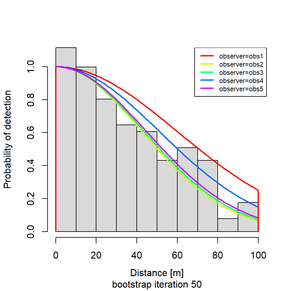
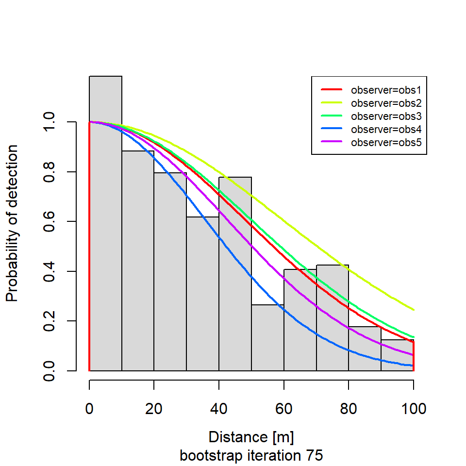
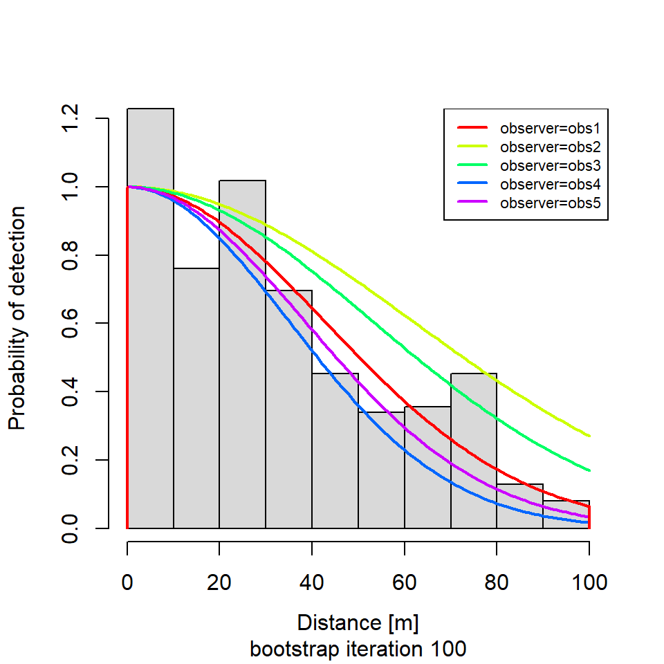
  # For the tutorial, plot the detection function of 5 iterations of the bootstrap
  if (i %in% round(seq(1, R, length.out = 5))) {
    plot(new.dfunc,
         newdata = data.frame(observer = unique(levels(new.sparrowSiteData$observer))),
         sub = paste0("bootstrap iteration ", i))
  }
  
  # Re-estimate abundance by site
  # and convert density to sparrows per 1 ha
  new.abundBySite <- predict(new.dfunc,
                             type = "abundance") |>
    mutate(density = set_units(density, "1/ha"),
           effort = set_units(effort, "ha"))
  
  # Re-create offset term and
  # Re-append site-level covariates
  new.abundBySite <- new.abundBySite |>
    mutate(offsetTerm = as.numeric(avgPdetect * effort)) |>
    left_join(new.sparrowSiteData,
              by = join_by(siteIDBoot))
  
  # Re-fit the (same) GLM
  new.pmod <- glm(individualsSeen ~ shrub + offset(log(offsetTerm)),
                  data = new.abundBySite,
                  family = "poisson")
  if( i <= 1 ){
    cat(paste0("---- New abundance model (iteration ", i, ")\n"))
    print(summary(new.pmod)$coefficients)
  }
  
  # Store regression coefficients
  b0[i] <- coef(new.pmod)[1]  # intercept
  b1[i] <- coef(new.pmod)[2]  # slope for shrub
  
}  # end bootstrap

---- Sites in Bootstrap 1

A1 A2 A3 A4 B1 B2 B3 B4 C1 C2 C3 C4 D1 D2 D3 D4 E1 E2 E3 E4 F1 F2 F3 F4 G1 G2 
 3  2  1  1  0  1  1  2  1  0  1  1  2  0  1  0  0  1  0  2  1  1  0  2  1  5 
G3 G4 H1 H2 H3 H4 I1 I2 I3 I4 J1 J2 J3 J4 K1 K2 K3 K4 L1 L2 L3 L4 M1 M2 M3 M4 
 3  2  0  0  0  1  0  2  3  1  0  0  0  1  0  0  1  2  1  2  0  2  1  1  1  0 
N1 N2 N3 N4 O1 O2 O3 O4 P1 P2 P3 P4 Q1 Q2 Q3 Q4 R1 R2 R3 R4 
 0  1  2  1  0  1  0  5  0  0  0  1  1  0  1  2  1  1  0  1 
---- New Site Data (iteration 1)
# A tibble: 6 × 9
  siteIDBoot siteID length observer  bare  herb shrub height shrubclass
  <chr>      <fct>     [m] <fct>    <dbl> <dbl> <dbl>  <dbl> <fct>     
1 A1.1       A1        500 obs4      36.7  15.9  20.1   26.4 High      
2 A1.2       A1        500 obs4      36.7  15.9  20.1   26.4 High      
3 A1.3       A1        500 obs4      36.7  15.9  20.1   26.4 High      
4 A2.1       A2        500 obs4      38.7  16.1  19.3   25   High      
5 A2.2       A2        500 obs4      38.7  16.1  19.3   25   High      
6 A3.1       A3        500 obs5      37.7  18.8  19.8   27   High      
---- New Detection Data (iteration 1)
# A tibble: 6 × 5
  siteIDBoot groupsize sightdist sightangle dist
  <chr>          <int>     <int>      <int>  [m]
1 A1.1               1        65         15 16.8
2 A1.1               1        70         10 12.2
3 A1.1               1        25         75 24.1
4 A1.1               1        40          5  3.5
5 A1.1               1        70         85 69.7
6 A1.1               1        10         90 10  
---- New Rdistance Data (iteration 1)
# A tibble: 6 × 10
# Rowwise:  siteIDBoot
  siteIDBoot         detections siteID length observer  bare  herb shrub height
  <chr>      <list<tibble[,4]>> <fct>     [m] <fct>    <dbl> <dbl> <dbl>  <dbl>
1 A1.1                 [15 × 4] A1        500 obs4      36.7  15.9  20.1   26.4
2 A1.2                 [15 × 4] A1        500 obs4      36.7  15.9  20.1   26.4
3 A1.3                 [15 × 4] A1        500 obs4      36.7  15.9  20.1   26.4
4 A2.1                 [13 × 4] A2        500 obs4      38.7  16.1  19.3   25  
5 A2.2                 [13 × 4] A2        500 obs4      38.7  16.1  19.3   25  
6 A3.1                 [10 × 4] A3        500 obs5      37.7  18.8  19.8   27  
# ℹ 1 more variable: shrubclass <fct>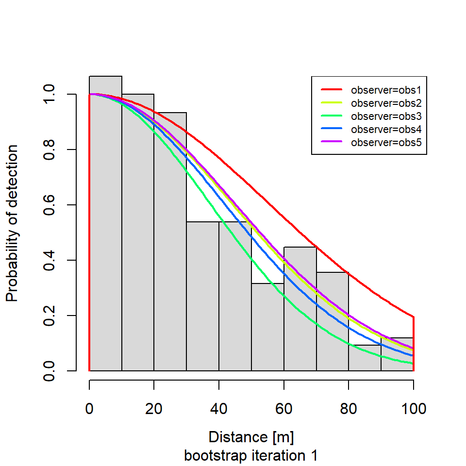

---- New abundance model (iteration 1)
               Estimate  Std. Error   z value     Pr(>|z|)
(Intercept) -1.18772590 0.141782244 -8.377113 5.424171e-17
shrub        0.09731473 0.009421497 10.329009 5.209592e-25

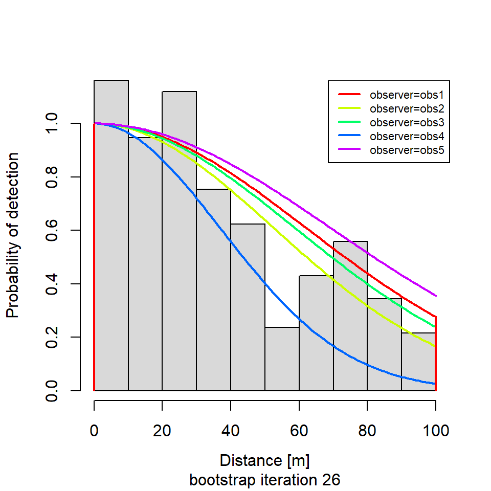
We now have a distribution for each of the regression coefficients in the Poisson GLM abundance model. If done correctly, the mean estimate from the bootstrap (solid black line, Figure 3 and Figure 4) should be very similar to the estimate from the original data (dotted blue line, Figure 3 and Figure 4). A 95% CI for each regression coefficient is estimated using the quantiles of the distribution (dashed black lines, Figure 3 and Figure 4).

hist(b0, breaks = 20, col = "grey", main = "Intercept (b0)")
abline(v = mean(b0), lwd = 2)
abline(v = coef(pmod)[1], col = "blue", lwd = 3, lty = "dotted")
abline(v = quantile(b0, c(0.025, 0.975)), lwd = 1.5, lty = "dashed")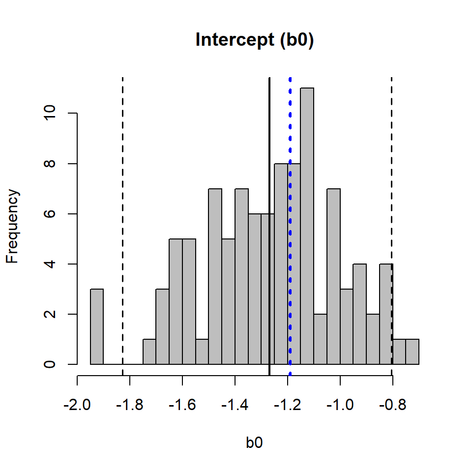

Figure 3: Bootstrap distribution of the regression’s intercept coefficient.

hist(b1, breaks = 20, col = "grey", main = "Shrub (b1)")
abline(v = mean(b1), lwd = 2)
abline(v = coef(pmod)[2], col = "blue", lwd = 3, lty = "dotted")
abline(v = quantile(b1, c(0.025, 0.975)), lwd = 1.5, lty = "dashed")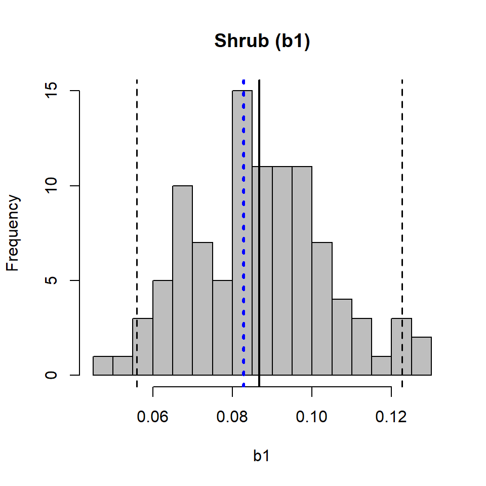

Figure 4: Bootstrap distribution of the regression’s slope coefficient.

It is interesting to remake Figure 2 based on the bootstrap results and show regression lines estimated during each iteration of the bootstrap (i.e., Figure 5 below). Based on those replicate regression lines, we calculate point-wise CIs for the original regression line. These CIs give an honest accounting of the uncertainty in the overall analysis because they include the uncertainty in both the detection and abundance stages (Buckland et al. 2009).

plot(abundBySite$density ~ abundBySite$shrub,
     xlab = "Shrub Cover (%)",
     ylab = "Sparrow Density (birds/ha)")

lines(predData$shrub, predData$densityEst, col = "black", lwd = 3)

for (i in 1:R) {
  lines(predData$shrub,
        exp(b0[i] + (b1[i]*predData$shrub)),
        col = "grey",
        lwd = 0.5)
}

xVals <- seq(min(abundBySite$shrub), max(abundBySite$shrub), length.out = 100)
bootLow <- rep(NA, length(xVals))
bootUpp <- rep(NA, length(xVals))

for (i in 1:length(xVals)) {
  y <- rep(NA, R)
  for (j in 1:R) {
    y[j] <- exp(b0[j] + (b1[j]*xVals[i]))
  }
  bootLow[i] <- quantile(y, 0.025)
  bootUpp[i] <- quantile(y, 0.975)
}

lines(xVals, bootLow, col = "black", lwd = 2, lty = "dashed")
lines(xVals, bootUpp, col = "black", lwd = 2, lty = "dashed")
lines(predData$shrub, predData$densityEst, col = "black", lwd = 3)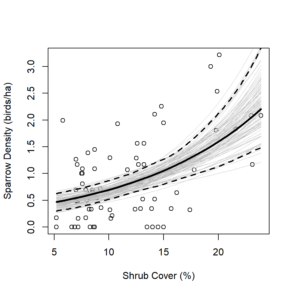

Figure 5: Scatterplot showing estimated relationship between schrub cover and sparrow density (black line), individual bootstrap iterations (gray lines), and point-wise confidence intervals derived during the two-stage process.

4 Results Comparison

Finally, we bring the results together to illustrate the point that conducting a two-stage analysis without properly propagating uncertainty via the bootstrap produces CI’s that are artificially narrow (red, Figure 6). Proper application of the two-stage bootstrap approach produces wider, more-honest, CIs (black, Figure 6).

plot(abundBySite$density ~ abundBySite$shrub,
     xlab = "Shrub Cover (%)",
     ylab = "Sparrow Density (birds/ha)")
lines(predData$shrub, predData$densityEst, col = "black", lwd = 3)
lines(predData$shrub, predData$lwr, col = "red", lwd = 2, lty = "dashed")
lines(predData$shrub, predData$upr, col = "red", lwd = 2, lty = "dashed")
lines(xVals, bootLow, col = "black", lwd = 2, lty = "dashed")
lines(xVals, bootUpp, col = "black", lwd = 2, lty = "dashed")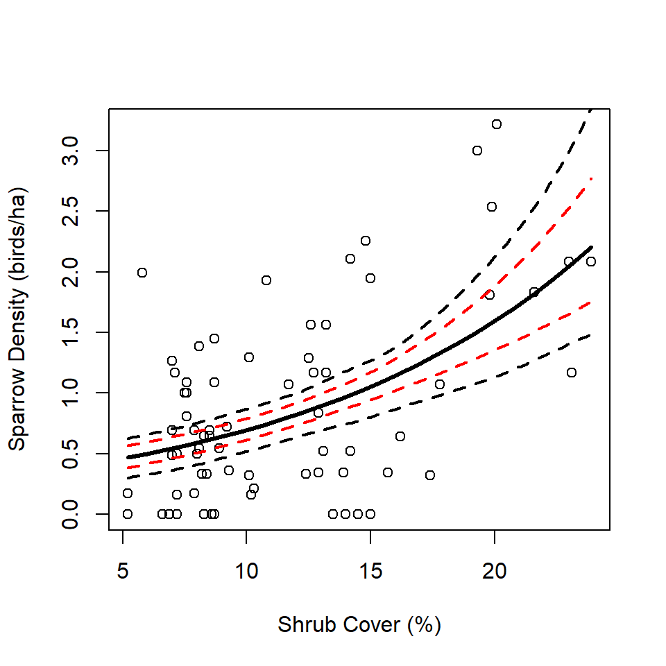

Figure 6: Final scatterplot showing non-bootstrap single-stage confidence intervals (red dashed line) and bootstrap two-stage confidence intervals.

Proper inflation of the CI’s afforded by the bootstrap is also evident in the regression coefficient CI’s.

confint(pmod, level = 0.95)

Waiting for profiling to be done...

                  2.5 %     97.5 %
(Intercept) -1.47419714 -0.9108982
shrub        0.06328019  0.1020780

ci.b0 <- quantile(b0, c(0.025, 0.975))
ci.b1 <- quantile(b1, c(0.025, 0.975))
                  
matrix(
  c(ci.b0,
    ci.b1), 
  nrow = 2, 
  byrow = TRUE,
  dimnames = list(c("(Intercept)", "shrub"), 
                  names(ci.b0))
)

                   2.5%      97.5%
(Intercept) -1.82699007 -0.8058737
shrub        0.05599327  0.1225509

Conclusion

We used Rdistance to estimate site-level abundance and accounted for imperfect detection. We then used the modeling framework of our choice to relate site-level covariates to abundance (or density). We demonstrated the workflow of this so-called two-stage approach using Rdistance by fitting a detection function that included observer, and regressed transect-specific density on shrub cover using a standard Poisson glm model. We also demonstrated proper use of a bootstrapping routine to appropriately propagate uncertainty from the detection stage of the analysis to the abundance stage.

References

Buckland, S. T., D. R. Anderson, K. P. Burnham, J. L. Laake, D. L. Borchers, and L. Thomas. 2001. Introduction to distance sampling: estimating abundance of biological populations. Oxford University Press, Oxford.

Buckland, S. T., R. E. Russell, B. G. Dickson, V. A. Saab, D. N. Gorman, and W. M. Block. 2009. Analyzing designed experiments in distance sampling. Journal of Agricultural, Biological, and Environmental Statistics 14(4):432-442.

Buckland, S. T., E. A. Rexstad, T. A. Marques, and C. S. Oedekoven. 2015. Distance sampling: methods and applications. Springer, New York, NY.

Carlisle, J. D., and A. D. Chalfoun. 2020. The abundance of Greater Sage-Grouse as a proxy for the abundance of sagebrush-associated songbirds in Wyoming, USA. Avian Conservation and Ecology 15(2):16. https://doi.org/10.5751/ACE-01702-150216.

Efron, B. 1979. Bootstrap methods: another look at the jackknife. Annals of Statistics 7:1-26.

Fiske, I. J., and R. B. Chandler. 2011. unmarked: an R package for fitting hierarchical models of wildlife occurrence and abundance. Journal of Statistical Software 43(10):1–23.

Gu, W., and R. K. Swihart. 2004. Absent or undetected? Effects of non-detection of species occurrence on wildlife-habitat models. Biological Conservation 116(2):195–203.

Kellner, K. F., A. D. Smith, J. A. Royle, M. Kéry, J. L. Belant, and R. B. Chandler. 2023. The unmarked R package: Twelve years of advances in occurrence and abundance modelling in ecology. Methods in Ecology and Evolution 14(6):1408–1415.

Kéry, M., and J. A. Royle. 2016. Applied hierarchical modeling in ecology: analysis of distribution, abundance, and species richness in R and BUGS. Academic Press, Amsterdam.

Kéry, M., and M. Schaub. 2012. Bayesian population analysis using WinBUGS: a hierarchical perspective. Academic Press, Waltham, MA.

Manly, B.F.J., and J.A. Navarro Alberto. 2020. Randomization, bootstrap and Monte Carlo methods in biology. 4th edition. CRC Press, Boca Raton, LA.

Marques, T. A., L. Thomas, M. Kéry, S. T. Buckland, D. L. Borchers, E. Rexstad, R. M. Fewster, D. I. MacKenzie, J. A. Royle, G. Guillera-Arroita, C. M. Handel, D. C. Pavlacky Jr., and R. J. Camp. 2017. Model-based approaches to deal with detectability: a comment on Hutto (2016a). Ecological Applications 27(5):1694–1698. http://doi.wiley.com/10.1002/eap.1553.

Schmidt, B. R., S. S. Cruickshank, C. Bühler, and A. Bergamini. 2023. Observers are a key source of detection heterogeneity and biased occupancy estimates in species monitoring. Biological Conservation 283(2023):110102. https://doi.org/10.1016/j.biocon.2023.110102.

Zuur, A. F., E. N. Ieno, N. J. Walker, A. A. Saveliev, and G. M. Smith. 2009. Mixed effects models and extensions in ecology with R. Springer Science & Business Media, New York, NY.