Effective Sample Distance 2: CIs for Specific Values
Confidence intervals for specific effective sampling distances
Advanced
Author
Trent L. McDonald
Published
September 24, 2025
Modified
December 5, 2025
Introduction
A previous tutorial, Effective Sample Distance 1, demonstrated confidence interval estimation for average effective sample distance (ESD). Confidence intervals for average ESD provide researchers with a reasonable ESD range and can be important for study planning or recognizing changes in detection probabilities. By definition, average ESD amalgomates ESD values over all covariate values. If, for example, detection differs between two observers, average ESD will fall somewhere between the individual ESDs.
NoteEffective Sample Distance
Effective Sample Distance (ESD) is the distance at which observers miss nearby targets as often as they find targets farther away. It is the distance at which missed targets offset included targets, and can be thought of as the effective distance of 100% detection. ESD plays a key role in density estimation. ESD can be off-transect distance, which we call Effective Strip Width (ESW), or radial distance from an observer, which we call Effective Detection Radius (EDR).
While useful in some cases, average ESD is not interesting in other cases. In some cases researchers would like ESD associated with specific values of detection covariates. For example, researchers might compare effective distances among observers, or in shrub and forest habitat. Rdistance’s effectiveDistance() function makes ESD point estimation easy when its newdata parameter is a data frame containing prediction covariate values.
But, what about a reasonable range for ESD point estimates? Variation in ESD would be useful if, for example, researchers plan transects in both shrub and forest habitat and they desire an estimate of the proportion of their study area they “effectively” cover. In these cases, confidence intervals on specific ESD values are needed, and the question is, “How do I do that?” How do we place a confidence interval on ESD associated with specific covariate values?
Unfortunately, confidence interval estimation for specific ESD is not easy in Rdistance (this was pointed out to the author in a recent email from an Rdistance user). The good news is that such confidence intervals are feasible. The not-so-good news is that these confidence intervals require a customized bootstrap loop like the one in this tutorial (Section 3, Listing 2).
Purpose
Demonstrate bootstrap confidence interval estimation for ESD associated with specific covariate values.
Note
The customized bootstrap loop used in this tutorial is not built into Rdistance. To use this method, analysts must cut and paste code from Listing 2 and Listing 3 (Section 3) into a local text file (e.g., in RStudio, press Ctrl-Shift-n to create a fresh .R script, and paste code there) and either run it line-by-line (Ctrl-Enter) or all at once (Ctrl-Shift-s).
Note
At the time of writing, this tutorial used a development version of Rdistance, i.e., version 4.1.0 (2025-08-21). The current CRAN version (4.0.5; 2025-04-10) works equally well with only minor output differences.
1 Base Distance Function Estimation
This tutorial follows Part 1 by fitting a distance function to Rdistance’s Brewer’s sparrow data that includes observer.
library(Rdistance)
Loading required package: units
udunits database from C:/Users/trent/AppData/Local/R/win-library/4.5/units/share/udunits/udunits2.xml
Rdistance (v4.1.0)
data("sparrowDf") # pull pre-defined Rdistance data frame to workspacetenHectares <- units::set_units(10, "ha") # pretend study area sizewhi <- units::set_units(200, "m") # right cutoff
The following statements estimate and summarize the distance function.
Call: dfuncEstim(data = sparrowDf, dist ~ observer +
   groupsize(groupsize), likelihood = "hazrate", w.hi = whi)
Coefficients:
              Estimate     SE         z           p(>|z|)
(Intercept)    3.97923469  0.1289595  30.8564643  4.587821e-209
observerobs2   0.19457534  0.1687260   1.1532029   2.488271e-01
observerobs3   0.05063578  0.1408215   0.3595741   7.191656e-01
observerobs4  -0.37709138  0.1588333  -2.3741329   1.759022e-02
observerobs5  -0.10615066  0.1478300  -0.7180590   4.727209e-01
k              3.25594658  0.3646960   8.9278381   4.344146e-19

Message: Success; Asymptotic SE's
Function: HAZRATE
Strip: 0 [m] to 200 [m]
Average effective strip width (ESW): 67.04909 [m] (range 47.674 [m] to 82.80148 [m])
Average probability of detection: 0.3352454 (range 0.23837 to 0.4140074)
Scaling: g(0 [m]) = 1
Log likelihood: -1642.054
AICc: 3296.35

     Surveyed Units: 36000 [m]
   Individuals seen: 372 in 354 groups
 Average group size: 1.050847
   Group size range: 1 to 3
Density in sampled area: 7.900855e-05 [1/m^2]
Abundance in 1e+05 [m^2] study area: 7.900855
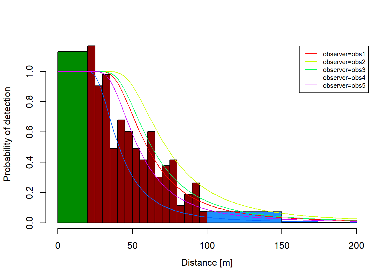
For good measure, we usually plot the estimated function on top of a histogram of observed distances. The following code demonstrates that Rdistance’s plot method allows users to specify arbitrary histogram bins to, for example, hightlight the steeper sections where detection drops quickly.
Figure 1: An estimated distance function relating Brewer’s sparrow observation distances (histogram bars) to individual observers (colored lines).
2 ESD For Specific Covariate Values
The ESD (an Effective Strip Width or ESW in this case) for each observer can be computed by calling effectiveDistance and specifying a newdata argument. The newdata argument is a data frame containing coavariate values at which to predict effective distances. Usage of newdata in Rdistance is identical in purpose as usage of newdata in base R’s lm, glm, gam, etc. (Note that we already used a newdata argument in the plot statement above to produce the five lines in Figure 1.)
The following code computes point estimates of effective distance for each observer.
ESD varies from 47.7 (obs4) to 82.8 (obs2) in this example. We compute confidence intervals for these numbers in Section 3 (Listing 2 and 3).
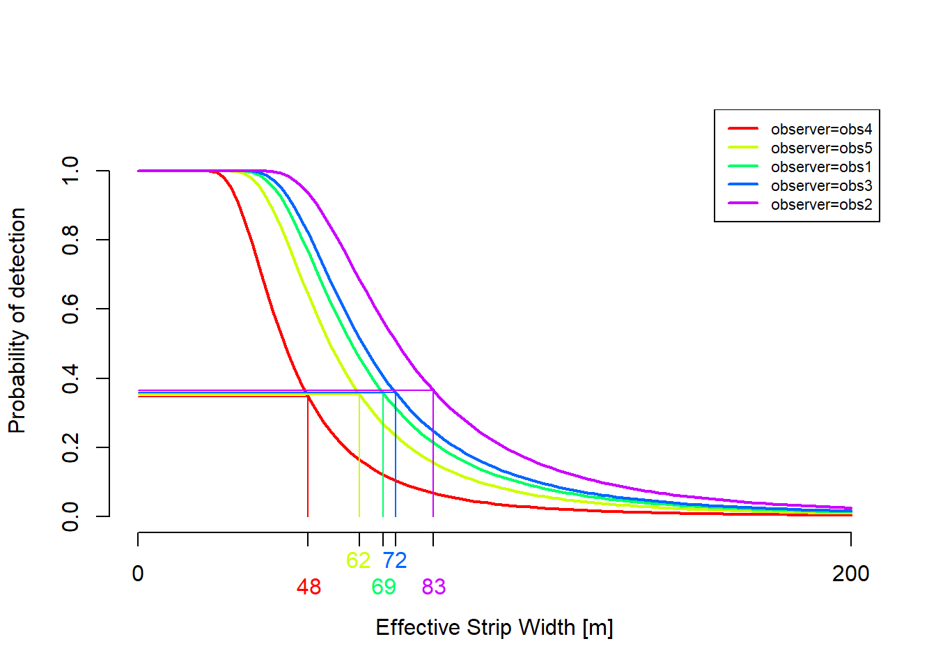
To illustrate ESD, the following plot shows observer-specific estimated distance functions and delineates each curve’s ESD.
Warning
Creating Figure 2, with its custom axis ticks and colors, is a bit complicated and is not really appropriate for R newbies. The main purpose for including this plot is to show the location of each curve’s ESD location and probability of detection at the ESD. Probability of detection at ESD is obtained by calling Rdistance’s predict method.
# Reorder by ESD for plottingord <-order(observerESD$esw)observerESD <- observerESD[ord, ] observers <- observers[ord,,drop=FALSE]# Plot distance functions and identify ESDmyCols <-rainbow(nrow(observerESD))plot(dfuncFit , newdata = observers , plotBars =FALSE , col = myCols , vertLines = F , xaxt ="n" , xlab ="Effective Strip Width [m]")axis(1 , tick =TRUE , at=c(0, observerESD$esw, 200) , labels =FALSE )axis(1 , tick =FALSE , at=c(0, 200) )dfuncHeights <-predict(dfuncFit , type ="dfuncs" , newdata = observers , distances = observerESD$esw ) # height of curves @ ESDfor( i in1:nrow(observerESD) ){axis(1 , at =round(observerESD$esw[i]) , line = (i %%2) -0.5 , tick =FALSE , col.axis = myCols[i] )lines(rep(observerESD$esw[i], 2) , c(0,dfuncHeights[i,i]) , col = myCols[i] )lines(c(0, observerESD$esw[i]) , rep(dfuncHeights[i,i], 2) , col = myCols[i] )}
Figure 2: Detection functions associated with observers in the example, and the probability of detection at their effective sampling distances.
NoteAside
In Figure 2, the probability of detection (height of the curve) at ESD varies slightly among observers. Probability of detection at ESD varies slightly because ESD is the area under each curve from left truncation to right truncation distance (here, 0 to 200) and this interval is fixed. To balance the number of detections at distances less than the ESD and the number of detections beyond ESD, the probability of detection at ESD must change slightly because the interval 0 to 200 is does not change. If we could integrate from 0 to infinity, curve heights at ESD would be equal; but, this makes no sense because ESD does not exist (i.e., is itself infinite) in this case.
3 Confidence Intervals
Confidence interval construction for the ESD point estimates associated with each observer requires a custom bootstrap loop (Listing 2), followed by summarization (Listing 3). The general algorithm for the bootstrap loop is,
Resample transects with replacement until we obtain the same number as in the original data set.
Fit the distance function to bootrap data.
Compute ESD at the specific covariate values.
Store ESD values and repeat the above many times.
Compute CI’s by the percentile or bias-corrected method.
Note
The ability of compute CIs for specific ESDs will likely be added to a future Rdistance release, assuming interest remains high.
In practice, the custom bootstrap loop proceeds as follows (Readers are encouraged run Listing 2 one-line-at-a-time and inspect the intermediate results):
Make a data frame containing the covariate values of interest (newDf below).
Make a data frame containing the original ESD estimates and their associated covariate values (origEsts below).
Write a bootstrap function that will be applied to every bootstrap data set. There are many ways to write this function. The function implemented below (estESW) takes the bootstrap identifier, random row indices, a data frame containing the covariate values of interest, and the original fitted object. It computes and returns a data frame containing ESD for each observer.
Construct a data frame containing “bootstrap indices” (bsIndices below). This data frame randomly samples, with replacement, the row indices of the original data, which in turn determines the rows in each bootstrap iteration (recall, each row in the original data frame represents one transect).
Use dplyr::group_modify to evaluate the bootstrap function on each bootstrap sample. dplyr::group_modify produces a giant data frame containing x rows for each of R bootstrap iterations (for a total of R\(\times\)x rows), where x is the number of rows returned by the bootstrap function.
Warning
Because ‘observer’ contains 5 levels (4 coefficients), bootstrap estimation is slow. 500 iterations took well over an hour on an otherwise fast desktop. Planned updates to ‘Rdistance’ should speed calculation considerably. Until then, patience is required.
Listing 2: R code implementing the custom bootstrap loop for computing confidence intervals on specific ESD values.
# Covariate values to predict at ----# 'observer' set in a previous code blocknewDf <- observers# The original point estimates ----# 'observerESD' set in a previous code blockorigEsts <- observerESD |> dplyr::rename(origESW = esw)# The 'bootstrap function' ----# A function applied to each BS sample estESW <-function(indexDf , key , data , newData , fit){# the BS sample bsdf <- data[indexDf$rowIndex,] # estimate distance function using BS data dfunc.bs <- Rdistance::dfuncEstim(data = bsdf , formula =formula(fit) , likelihood = fit$likelihood , w.lo = fit$w.lo , w.hi = fit$w.hi# + other options, e.g., x.scl )# estimate ESD for specific covariates, and return eswBS <- Rdistance::effectiveDistance(object = dfunc.bs , newdata = newData ) eswBS <-cbind(newData, data.frame(ESW = eswBS))return(eswBS) }# Prepare bootstrap indices ----R <-500# number of BS interationsnDigits <-ceiling(log10(R +1)) # max digits in indexnDataRows <-nrow(sparrowDf) # number of transectsid <-rep(1:R, each = nDataRows) bsIndices <-data.frame(id =paste0("Bootstrap_",formatC(id , format ="f" , digits =0 , width = nDigits , flag ="0")) , rowIndex =sample( 1:nDataRows , size = R*nDataRows , replace =TRUE ))# In bsIndicies: 'id' is BS iteration number; 'rowIndex' is# row in original data data set# Apply 'bootstrap function' to ID groups using dplyr::group_modify ----eswB <- bsIndices |> dplyr::group_by(id) |> dplyr::group_modify(.f = estESW # BS function , data = sparrowDf # the original , newData = newDf # covariates , fit = dfuncFit # the original )
When finished, data frame eswB contains one value of id for each bootstrap iteration, and each bootstrap iteration contains five predicted ESD values, one for each observer.
We compute bootstrap confidence intervals, after re-grouping (by observer in this case), by calling functions that return either the lower or upper endpoint of the interval. The following code demonstrates computation of both the percentile and bias-corrected bootstrap intervals. In this case, the author leans toward reporting bias-corrected bootstrap intervals because the distribution of ESD is not very skewed (see e.g., x <- dplyr::filter(eswB, observer == "obs4"); hist(x)).
Listing 3: Calculation of percentile and bias-corrected confidence interval endpoints on results of the bootstrap loop.
# Regroup BS data by covariate values ----eswB <- eswB |> dplyr::group_by(dplyr::across(dplyr::all_of(names(newDf))))# Merge in original point estimates b/c bias corrected ----# intervals require the originals eswB <- eswB |> dplyr::left_join(origEsts, by =names(newDf))# Compute both percentile and bias-corrected intervals ----eswCI <- eswB |> dplyr::summarise(pt_eswLo95 =quantile(ESW, p =0.025) # Percentile Low , pt_eswHi95 =quantile(ESW, p =0.975) # Percentile High , bc_eswLo95 = Rdistance::bcCI(x.bs = ESW , x = origESW[1] , ci =0.95)[1] # BiasCorr Low , bc_eswHi95 = Rdistance::bcCI(x.bs = ESW , x = origESW[1] , ci =0.95)[2] # BiasCorr High ) finalAnswer <- origEsts |> dplyr::full_join(eswCI, by =names(newDf))finalAnswer
Interval endpoints differ by less than 3 [m] between methods in this case (compare columns pt_esw??95 to bc_esw??95). The author deems these differences immaterial and opts for the bias-corrected version. The final, nicely formatted, intervals for observer ESD appear in Table 1.
Table 1: Final point estimates and 95% bias-corrected bootstrap confidence intervals for observer effective strip width, sorted from shortest to longest.
Observer
ESW (95% CI)
obs4
47.7 (38.9, 60.4)
obs5
62.1 (51.5, 80.9)
obs1
68.8 (57, 99.4)
obs3
72.2 (37.6, 88.9)
obs2
82.8 (63.5, 117.3)
In this example, Observer 4’s confidence interval does not overlap that of Observer 2. While this is not a formal test of ESD differences, it is pretty close. A formal (bootstrap) test for differences among ESD requires bootstrap sampling under the null hypothesis of equality and is outside the scope of this tutorial (perhaps it will be the topic of a future tutorial).
Final Notes
The bootstrap method demonstrated here is fairly general. Analysts can place confidence intervals on other derived parameters of distance functions by changing the output of the bootstrap function (estESW above). For example, the bootstrap function could return:
A linear combination of distance function coefficients
The probability of detection at a particular distance
Mean ESD over sub-sets of the covariate values
To illustrate the last point, suppose detections were collected using multiple walking transect types (e.g., two vs. one observer; trials vs. bushwhacking; slow vs. fast). Analysts could modify the bootstrap function to average ESD over two or more types while fitting all types in the base distance function.